Documentation

• 1: Formatting Tips
• 1.1: Formatting Tips
• 1.2: Diagrams and Formulae
• 2: Class Contents
• 2.1: Tohoku Univ.
• 2.1.1: Specialized Education
• 2.1.1.1: Exercise in Mathematics and Physics Ⅱ
• 2.1.1.1.1: Chapter 25 Solutions
• 2.1.1.1.2: Chapter 26 Solutions
• 2.1.1.2: Mathematics Ⅱ
• 2.1.1.2.1: 4 - Fourier Transform
• 2.1.1.2.2: 5 - PDE
• 2.1.2: General Education
• 3: General Notes
• 3.1: Personal Mathematics

1 - Formatting Tips

1.1 - Formatting Tips

Text can be bold, italic, or strikethrough. Links should be blue with no underlines (unless hovered over).

Blockquotes should be a lighter gray with a border along the left side in the secondary color.

Header 2 (Header 1 is for title.)

This is a blockquote following a header. Bacon ipsum dolor sit amet t-bone doner shank drumstick, pork belly porchetta chuck sausage brisket ham hock rump pig. Chuck kielbasa leberkas, pork bresaola ham hock filet mignon cow shoulder short ribs biltong.

Header 3

This is a code block following a header.

Header 4

• This is an unordered list following a header.
• This is an unordered list following a header.
• This is an unordered list following a header.

1. This is an ordered list following a header.
2. This is an ordered list following a header.
3. This is an ordered list following a header.

Header 5

And an unordered task list:

• Create a sample markdown document
• Add task lists to it
• Take a vacation

And a nested list:

• Jackson 5
  • Michael
  • Tito
  • Jackie
  • Marlon
  • Jermaine
• TMNT
  • Leonardo
  • Michelangelo
  • Donatello
  • Raphael

Header 6

There’s a horizontal rule above and below this.

Definition lists can be used with Markdown syntax. Definition terms are bold.

Name

Godzilla

Born

1952

Birthplace

Japan

Color

Green

Tables should have bold headings and alternating shaded rows.

If a table is too wide, it should scroll horizontally.

Code snippets like var foo = "bar"; can be shown inline. Also, this should vertically align with this and this.

Code can also be shown in a block element.

foo := "bar";
bar := "foo";

Code can also use syntax highlighting.

func main() {
  input := `var foo = "bar";`

  lexer := lexers.Get("javascript")
  iterator, _ := lexer.Tokenise(nil, input)
  style := styles.Get("github")
  formatter := html.New(html.WithLineNumbers())

  var buff bytes.Buffer
  formatter.Format(&buff, style, iterator)

  fmt.Println(buff.String())
}

Long, single-line code blocks should not wrap. They should horizontally scroll if they are too long. This line should be long enough to demonstrate this.

Inline code inside table cells should still be distinguishable.

Small images should be shown at their actual size.

Large images should always scale down and fit in the content container.

Components

Alerts

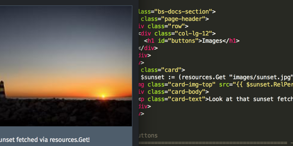
Including images

Here’s an image (featured-sunset-get.png) that includes a byline and a caption.

The front matter of this post specifies properties to be assigned to all image resources:

resources:
- src: "**.{png,jpg}"
  title: "Image #:counter"
  params:
    byline: "Photo: Riona MacNamara / CC-BY-CA"

To include the image in a page, specify its details like this:

The image will be rendered at the size and byline specified in the front matter.

This is the final element on the page and there should be no margin below this.

@chalin,¹

https://www.cncf.io/blog/2023/06/05/migrating-docsy-to-bootstrap-5/

1.2 - Diagrams and Formulae

Docsy has built-in support for a number of diagram creation and typesetting tools you can use to add rich content to your site, including \(\KaTeX\), Mermaid, Diagrams.net, PlantUML, and MarkMap.

\(\LaTeX\) support with \(\KaTeX\)

\(\LaTeX\) is a high-quality typesetting system for the production of technical and scientific documentation. Due to its excellent math typesetting capabilities, \(\TeX\) became the de facto standard for the communication and publication of scientific documents, especially if these documents contain a lot of mathematical formulae. Designed and mostly written by Donald Knuth, the initial version was released in 1978. Dating back that far, \(\LaTeX\) has pdf as its primary output target and is not particularly well suited for producing HTML output for the Web. Fortunately, with \(\KaTeX\) there exists a fast and easy-to-use JavaScript library for \(\TeX\) math rendering on the web, which was integrated into the Docsy theme.

With \(\KaTeX\) support enabled in Docsy, you can include complex mathematical formulae into your web page, either inline or centred on its own line. Since \(\KaTeX\) relies on server side rendering, it produces the same output regardless of your browser or your environment. Formulae can be shown either inline or in display mode:

Inline formulae

The following code sample produces a text line with three inline formulae:

When \\(a \ne 0\\), there are two solutions to \\(ax^2 + bx + c= 0\\) and they are \\(x = {-b \pm \sqrt{b^2-4ac} \over 2a}\\).

When \(a \ne 0\), there are two solutions to \(ax^2 + bx + c= 0\) and they are \(x = {-b \pm \sqrt{b^2-4ac} \over 2a}\).

Formulae in display mode

The following code sample produces an introductory text line followed by a formula numbered as (1) residing on its own line:

The probability of getting \\(k\\) heads when flipping \\(n\\) coins is:
```math
\tag*{(1)} P(E) = {n \choose k} p^k (1-p)^{n-k}
```

The formula itself is written inside a GLFM math block. The above code fragment renders to:

The probability of getting \(k\) heads when flipping \(n\) coins is:

$$
\tag*{(1)} P(E) = {n \choose k} p^k (1-p)^{n-k}
$$

Activating and configuring \(\KaTeX\) support

Auto activation

As soon as you use a math code block on your page, support of \(\KaTeX\) is automatically enabled.

Manual activation (no math code block present or hugo 0.92 or lower)

If you want to use inline formulae and don’t have a math code block present in your page which triggers auto activation, you need to manually activate \(\KaTeX\) support. The easiest way to do so is to add a math attribute to the frontmatter of your page and set it to true:

• Page front matter:
• toml
• yaml
• json

+++
math = true
+++

---
math: true
---

{
  "math": true
}

If you use formulae in most of your pages, you can also enable sitewide \(\KaTeX\) support inside the Docsy theme. To do so update hugo.toml/hugo.yaml/hugo.json:

• Site configuration file:
• hugo.toml
• hugo.yaml
• hugo.json

[params.katex]
enable = true

params:
  katex:
    enable: true

{
  "params": {
    "katex": {
      "enable": true
    }
  }
}

Additionally, you can customize various \(\KaTeX\) options inside hugo.toml/hugo.yaml/hugo.json, if needed:

• Site configuration file:
• hugo.toml
• hugo.yaml
• hugo.json

[params.katex]
# enable/disable KaTeX support
enable = true
# Element(s) scanned by auto render extension. Default: document.body
html_dom_element = "document.body"

[params.katex.options]
# If true (the default), KaTeX will throw a ParseError when it encounters an
# unsupported command or invalid LaTeX. If false, KaTeX will render unsupported
# commands as text, and render invalid LaTeX as its source code with hover text
# giving the error, in the color given by errorColor.
throwOnError = false
errorColor = "#CD5C5C"

# This is a list of delimiters to look for math, processed in the same order as
# the list. Each delimiter has three properties:
#   left:    A string which starts the math expression (i.e. the left delimiter).
#   right:   A string which ends the math expression (i.e. the right delimiter).
#   display: Whether math in the expression should be rendered in display mode.
[[params.katex.options.delimiters]]
  left = "$$"
  right = "$$"
  display = true
[[params.katex.options.delimiters]]
  left = "$"
  right = "$"
  display = false
[[params.katex.options.delimiters]]
  left = "\\("
  right = "\\)"
  display = false
[[params.katex.options.delimiters]]
  left = "\\["
  right = "\\]"
  display = true

params:
  katex:
    enable: true  # enable/disable KaTeX support
    html_dom_element: document.body  # Element(s) scanned by auto render extension. Default: document.body
    options:

      # If true (the default), KaTeX will throw a ParseError when it encounters an
      # unsupported command or invalid LaTeX. If false, KaTeX will render unsupported
      # commands as text, and render invalid LaTeX as its source code with hover text
      # giving the error, in the color given by errorColor.
      throwOnError: false
      errorColor: '#CD5C5C'

      # This is a list of delimiters to look for math, processed in the same order as
      # the list. Each delimiter has three properties:
      #   left:    A string which starts the math expression (i.e. the left delimiter).
      #   right:   A string which ends the math expression (i.e. the right delimiter).
      #   display: Whether math in the expression should be rendered in display mode.
      delimiters:
        - left: $$
          right: $$
          display: true
        - left: $
          right: $
          display: false
        - left: \(
          right: \)
          display: false
        - left: \[
          right: \]
          display: true

{
  "params": {
    "katex": {
      "enable": true,
      "html_dom_element": "document.body",
      "options": {
        "throwOnError": false,
        "errorColor": "#CD5C5C",
        "delimiters": [
          {
            "left": "$$",
            "right": "$$",
            "display": true
          },
          {
            "left": "$",
            "right": "$",
            "display": false
          },
          {
            "left": "\\(",
            "right": "\\)",
            "display": false
          },
          {
            "left": "\\[",
            "right": "\\]",
            "display": true
          }
        ]
      }
    }
  }
}

For a complete list of options and their detailed description, have a look at the documentation of \({\KaTeX}\)’s Rendering API options and of \({\KaTeX}\)’s configuration options.

Display of Chemical Equations and Physical Units

mhchem is a \(\LaTeX\) package for typesetting chemical molecular formulae and equations. Fortunately, \(\KaTeX\) provides the mhchem extension that makes the mhchem package accessible when authoring content for the web. With mhchem extension enabled, you can easily include chemical equations into your page. An equation can be shown either inline or can reside on its own line. The following code sample produces a text line including a chemical equation:

*Precipitation of barium sulfate:* \\(\ce{SO4^2- + Ba^2+ -> BaSO4 v}\\)

Precipitation of barium sulfate: \(\ce{SO4^2- + Ba^2+ -> BaSO4 v}\)

More complex equations need to be displayed on their own line. Use a code block adorned with chem in order to achieve this:

```chem
\tag*{(2)} \ce{Zn^2+  <=>[+ 2OH-][+ 2H+]  $\underset{\text{amphoteric hydroxide}}{\ce{Zn(OH)2 v}}$  <=>[+ 2OH-][+ 2H+]  $\underset{\text{tetrahydroxozincate}}{\ce{[Zn(OH)4]^2-}}$}
```

$$
\tag*{(2)} \ce{Zn^2+  <=>[+ 2OH-][+ 2H+]  $\underset{\text{amphoteric hydroxide}}{\ce{Zn(OH)2 v}}$  <=>[+ 2OH-][+ 2H+]  $\underset{\text{tetrahydroxozincate}}{\ce{[Zn(OH)4]^2-}}$}
$$

Use of mhchem is not limited to the authoring of chemical equations, using the included \pu command, pretty looking physical units can be written with ease, too. The following code sample produces two text lines with four numbers plus their corresponding physical units:

* Scientific number notation: \\(\pu{1.2e3 kJ}\\) or \\(\pu{1.2E3 kJ}\\) \\
* Divisions: \\(\pu{123 kJ/mol}\\) or \\(\pu{123 kJ//mol}\\)

• Scientific number notation: \(\pu{1.2e3 kJ}\) or \(\pu{1.2E3 kJ}\)
• Divisions: \(\pu{123 kJ/mol}\) or \(\pu{123 kJ//mol}\)

For a complete list of options when authoring physical units, have a look at the section on physical units in the mhchem documentation.

Activating rendering support for chemical formulae

Auto activation

As soon as you use a chem code block on your page, rendering support for chemical equations is automatically enabled.

Manual activation (no chem code block present or hugo 0.92 or lower)

If you want to use chemical formulae inline and don’t have a chem code block present in your page which triggers auto activation, you need to manually activate rendering support for chemical formulae. The easiest way to do so is to add a chem attribute to the frontmatter of your page and set it to true:

• Page front matter:
• toml
• yaml
• json

+++
chem = true
+++

---
chem: true
---

{
  "chem": true
}

If you use formulae in most of your pages, you can also enable sitewide rendering support for chemical formulae inside the Docsy theme. To do so, enable mhchem inside your hugo.toml/hugo.yaml/hugo.json:

• Site configuration file:
• hugo.toml
• hugo.yaml
• hugo.json

[params.katex]
enable = true

[params.katex.mhchem]
enable = true

params:
  katex:
    enable: true
    mhchem:
      enable: true

{
  "params": {
    "katex": {
      "enable": true,
      "mhchem": {
        "enable": true
      }
    }
  }
}

Diagrams with Mermaid

Mermaid is a Javascript library for rendering simple text definitions to useful diagrams in the browser. It can generate a variety of different diagram types, including flowcharts, sequence diagrams, class diagrams, state diagrams, ER diagrams, user journey diagrams, Gantt charts and pie charts.

With Mermaid support enabled in Docsy, you can include the text definition of a Mermaid diagram inside a code block, and it will automatically be rendered by the browser as soon as the page loads.

The great advantage of this is anyone who can edit the page can now edit the diagram - no more hunting for the original tools and version to make a new edit.

For example, the following defines a sequence diagram:

```mermaid
sequenceDiagram
    autonumber
    Docsy user->>Discussion board: Ask question
    Discussion board->>Community member: read question
    loop Different strategies
    Community member->>Test instance: Investigate issue raised
    end
    Note right of Community member: After hours of investigation:
    Test instance-->>Community member: Come up with solution
    Community member-->>Discussion board: Propose solution
    Discussion board-->>Docsy user: check proposed solution
    Docsy user->>Discussion board: Mark question as resolved
    Docsy user->>Docsy user: Being happy
```

which is automatically rendered to:

sequenceDiagram
    autonumber
    Docsy user->>Discussion board: Ask question
    Discussion board->>Community member: read question
    loop Different strategies
    Community member->>Test instance: Investigate issue raised
    end
    Note right of Community member: After hours of investigation:
    Test instance-->>Community member: Come up with solution
    Community member-->>Discussion board: Propose solution
    Discussion board-->>Docsy user: check proposed solution
    Docsy user->>Discussion board: Mark question as resolved
    Docsy user->>Docsy user: Being happy

Support of Mermaid diagrams is automatically enabled as soon as you use a mermaid code block on your page.

By default, docsy pulls in the latest officially released version of Mermaid at build time. If that doesn’t fit your needs, you can specify the wanted mermaid version inside your configuration file hugo.toml/hugo.yaml/hugo.json:

• Configuration file:
• hugo.toml
• hugo.yaml
• hugo.json

[params.mermaid]
version = "10.9.0"

params:
  mermaid:
    version: 10.9.0

{
  "params": {
    "mermaid": {
      "version": "10.9.0"
    }
  }
}

If needed, you can define custom settings for your diagrams, such as themes, padding in your hugo.toml/hugo.yaml/hugo.json.

• Configuration file:
• hugo.toml
• hugo.yaml
• hugo.json

[params.mermaid]
theme = "neutral"

[params.mermaid.flowchart]
diagramPadding = 6

params:
  mermaid:
    theme: neutral
    flowchart:
      diagramPadding: 6

{
  "params": {
    "mermaid": {
      "theme": "neutral",
      "flowchart": {
        "diagramPadding": 6
      }
    }
  }
}

See the Mermaid documentation for a list of defaults that can be overridden.

Settings can also be overridden on a per-diagram basis by making use of a frontmatter config block at the start of the diagram definition.

UML Diagrams with PlantUML

PlantUML is an alternative to Mermaid that lets you quickly create UML diagrams, including sequence diagrams, use case diagrams, and state diagrams. Unlike Mermaid diagrams, which are entirely rendered in the browser, PlantUML uses a PlantUML server to create diagrams. You can use the provided default demo server (not recommended for production use), or run a server yourself. PlantUML offers a wider range of image types than Mermaid, so may be a better choice for some use cases.

Diagrams are defined using a simple and intuitive language. (see PlantUML Language Reference Guide).

The following example shows a use case diagram:

```plantuml
participant participant as Foo
actor       actor       as Foo1
boundary    boundary    as Foo2
control     control     as Foo3
entity      entity      as Foo4
database    database    as Foo5
collections collections as Foo6
queue       queue       as Foo7
Foo -> Foo1 : To actor
Foo -> Foo2 : To boundary
Foo -> Foo3 : To control
Foo -> Foo4 : To entity
Foo -> Foo5 : To database
Foo -> Foo6 : To collections
Foo -> Foo7: To queue
```

Automatically renders to:

participant participant as Foo
actor       actor       as Foo1
boundary    boundary    as Foo2
control     control     as Foo3
entity      entity      as Foo4
database    database    as Foo5
collections collections as Foo6
queue       queue       as Foo7
Foo -> Foo1 : To actor
Foo -> Foo2 : To boundary
Foo -> Foo3 : To control
Foo -> Foo4 : To entity
Foo -> Foo5 : To database
Foo -> Foo6 : To collections
Foo -> Foo7: To queue

To enable/disable PlantUML, update hugo.toml/hugo.yaml/hugo.json:

• Configuration file:
• hugo.toml
• hugo.yaml
• hugo.json

[params.plantuml]
enable = true

params:
  plantuml:
    enable: true

{
  "params": {
    "plantuml": {
      "enable": true
    }
  }
}

Other optional settings are:

• Configuration file:
• hugo.toml
• hugo.yaml
• hugo.json

[params.plantuml]
enable = true
theme = "default"

# Set url to plantuml server
# default is http://www.plantuml.com/plantuml/svg/
svg_image_url = "https://www.plantuml.com/plantuml/svg/"

# By default the plantuml implementation uses <img /> tags to display UML diagrams.
# When svg is set to true, diagrams are displayed using <svg /> tags, maintaining functionality like links e.g.
# default = false
svg = true

params:
  plantuml:
    enable: true
    theme: default
    # Set url to plantuml server
    # default is http://www.plantuml.com/plantuml/svg/
    svg_image_url: 'https://www.plantuml.com/plantuml/svg/'
    # By default the plantuml implementation uses <img /> tags to display UML diagrams.
    # When svg is set to true, diagrams are displayed using <svg /> tags, maintaining functionality like links e.g.
    # default = false
    svg: true

{
  "params": {
    "plantuml": {
      "enable": true,
      "theme": "default",
      "svg_image_url": "https://www.plantuml.com/plantuml/svg/",
      "svg": true
    }
  }
}

MindMap support with MarkMap

MarkMap is a Javascript library for rendering simple text definitions to MindMap in the browser.

For example, the following defines a simple MindMap:

```markmap
# markmap

## Links

- <https://markmap.js.org/>
- [GitHub](https://github.com/gera2ld/markmap)

## Related

- [coc-markmap](https://github.com/gera2ld/coc-markmap)
- [gatsby-remark-markmap](https://github.com/gera2ld/gatsby-remark-markmap)

## Features

- links
- **inline** ~~text~~ *styles*
- multiline
  text
- `inline code`
-
    ```js
    console.log('code block');
    ```
- Katex - $x = {-b \pm \sqrt{b^2-4ac} \over 2a}$
```

Automatically renders to:

# markmap

## Links

- <https://markmap.js.org/>
- [GitHub](https://github.com/gera2ld/markmap)

## Related

- [coc-markmap](https://github.com/gera2ld/coc-markmap)
- [gatsby-remark-markmap](https://github.com/gera2ld/gatsby-remark-markmap)

## Features

- links
- **inline** ~~text~~ *styles*
- multiline
  text
- `inline code`
-
    ```js
    console.log('code block');
    ```
- Katex - $x = {-b \pm \sqrt{b^2-4ac} \over 2a}$

To enable/disable MarkMap, update hugo.toml/hugo.yaml/hugo.json:

• Configuration file:
• hugo.toml
• hugo.yaml
• hugo.json

[params.markmap]
enable = true

params:
  markmap:
    enable: true

{
  "params": {
    "markmap": {
      "enable": true
    }
  }
}

Diagrams with Diagrams.net

Diagrams.net (aka draw.io) provides a free and open source diagram editor that can generate a wider range of diagrams than Mermaid or PlantUML using a web or desktop editor.

SVG and PNG files exported with the tool contain the source code of the original diagram by default, which allows the diagrams.net site to import those images again for edit in the future. With draw.io enabled, Docsy will detect this and automatically add an Edit button over any image that can be edited using the online site.

Hover over the image below and click edit to instantly start working with it. Clicking the Save button will cause the edited diagram to be exported using the same filename and filetype, and downloaded to your browser.

As the diagram data is transported via the browser, the diagrams.net server does not need to access the content on your Docsy server directly at all.

To enable detection of diagrams, update hugo.toml/hugo.yaml/hugo.json:

• Configuration file:
• hugo.toml
• hugo.yaml
• hugo.json

[params.drawio]
enable = true

params:
  drawio:
    enable: true

{
  "params": {
    "drawio": {
      "enable": true
    }
  }
}

You can also deploy and use your own server for editing diagrams, in which case update the configuration to point to that server:

• Configuration file:
• hugo.toml
• hugo.yaml
• hugo.json

[params.drawio]
drawio_server = "https://app.mydrawioserver.example.com"

params:
  drawio:
    drawio_server: 'https://app.mydrawioserver.example.com'

{
  "params": {
    "drawio": {
      "drawio_server": "https://app.mydrawioserver.example.com"
    }
  }
}

2 - Class Contents

2.1 - Tohoku Univ.

2.1.1 - Specialized Education

2.1.1.1 - Exercise in Mathematics and Physics Ⅱ

2.1.1.1.1 - Chapter 25 Solutions

Chapter 25 Solutions

1. Complex Trigonometric Equation

Problem

Find all complex numbers \(z\) which satisfy the equation \(\sin(z) = 5\).

Solution

We use the exponential definition of the sine function for a complex variable \(z = x + iy\):

Set this equal to 5:

To solve this, we make a substitution. Let \(w = e^{iz}\). Then \(e^{-iz} = \frac{1}{w}\). The equation becomes:

Multiply the entire equation by \(w\) to eliminate the fraction:

Rearrange this into a standard quadratic equation \(aw^2 + bw + c = 0\):

We solve for \(w\) using the quadratic formula \(w = \frac{-b \pm \sqrt{b^2 - 4ac}}{2a}\):

Now we have two possible values for \(w\). We must solve for \(z\) by substituting back \(w = e^{iz}\), which means \(iz = \log(w)\). Remember that the complex logarithm is multi-valued: \(\log(w) = \ln|w| + i(\arg(w) + 2n\pi)\) for \(n \in \mathbb{Z}\).

Case 1: \(w = (5 + 2\sqrt{6})i\)

\(|w| = 5 + 2\sqrt{6}\). The argument \(\arg(w)\) is \(\frac{\pi}{2}\) since it’s on the positive imaginary axis.

Multiply by \(\frac{1}{i} = -i\):

Case 2: \(w = (5 - 2\sqrt{6})i\)

\(|w| = 5 - 2\sqrt{6}\). The argument \(\arg(w)\) is also \(\frac{\pi}{2}\).

Multiply by \(\frac{1}{i} = -i\):

Note that \(\ln(5 - 2\sqrt{6}) = \ln\left(\frac{(5 - 2\sqrt{6})(5 + 2\sqrt{6})}{5 + 2\sqrt{6}}\right) = \ln\left(\frac{1}{5 + 2\sqrt{6}}\right) = -\ln(5 + 2\sqrt{6})\). So, this second case gives \(z = i \ln(5 + 2\sqrt{6}) + \left(\frac{\pi}{2} + 2n\pi\right)\).

We can combine both cases into a single expression:

4. Cauchy’s Integral Formula / Residue Theorem

Problem

For the path integral \(\oint_C \frac{z}{(z - 3)(z + 1 + i)} dz\), calculate its values at \(|z| = 1\) and \(|z| = 4\).

Solution

The integrand is \(f(z) = \frac{z}{(z - 3)(z - (-1 - i))}\). The function has two simple poles at \(z_1 = 3\) and \(z_2 = -1 - i\).

Case 1: C is the circle \(|z| = 1\)

We check if the poles lie inside the contour \(C\).

• For \(z_1 = 3\): \(|z_1| = |3| = 3\). Since \(3 > 1\), this pole is outside the contour.
• For \(z_2 = -1 - i\): \(|z_2| = |-1 - i| = \sqrt{(-1)^2 + (-1)^2} = \sqrt{2} \approx 1.414\). Since \(\sqrt{2} > 1\), this pole is also outside the contour.

Since the function \(f(z)\) is analytic everywhere inside and on the contour \(|z|=1\), by Cauchy’s Integral Theorem, the value of the integral is 0.

Case 2: C is the circle \(|z| = 4\)

We check if the poles lie inside this new contour.

• For \(z_1 = 3\): \(|z_1| = 3\). Since \(3 < 4\), this pole is inside the contour.
• For \(z_2 = -1 - i\): \(|z_2| = \sqrt{2}\). Since \(\sqrt{2} < 4\), this pole is also inside the contour.

Since both poles are inside, we use the Residue Theorem. The integral is \(2\pi i\) times the sum of the residues at the enclosed poles.

• Residue at \(z_1 = 3\):
  $$\text{Res}(f, 3) = \lim_{z\to 3} (z-3)f(z) = \lim_{z\to 3} \frac{z}{z+1+i} = \frac{3}{4+i}$$
  $$= \frac{3(4-i)}{(4+i)(4-i)} = \frac{12-3i}{16-i^2} = \frac{12-3i}{17}$$
• Residue at \(z_2 = -1 - i\):
  $$\text{Res}(f, -1-i) = \lim_{z\to -1-i} (z-(-1-i))f(z) = \lim_{z\to -1-i} \frac{z}{z-3} = \frac{-1-i}{-1-i-3} = \frac{-(1+i)}{-(4+i)} = \frac{1+i}{4+i}$$
  $$= \frac{(1+i)(4-i)}{(4+i)(4-i)} = \frac{4-i+4i-i^2}{17} = \frac{5+3i}{17}$$
• Sum of residues:
  $$\frac{12 - 3i}{17} + \frac{5 + 3i}{17} = \frac{17}{17} = 1$$

The value of the integral is \(2\pi i \times (\text{Sum of residues}) = 2\pi i \times 1 = \mathbf{2\pi i}\).

5. Path Integral on the Unit Circle

Problem

For the path integral \(\oint_C \frac{d\theta}{z + \cos\theta}\) calculate its value at \(|z| = 1\) (where \(z = e^{i\theta}, 0 \le \theta \le 2\pi\)).

Solution

We convert the entire integral into the \(z\) domain. The contour \(C\) is the unit circle.

• \(z = e^{i\theta}\)
• \(dz = i e^{i\theta} d\theta = iz d\theta \implies d\theta = \frac{dz}{iz}\)
• \(\cos\theta = \frac{e^{i\theta} + e^{-i\theta}}{2} = \frac{z + 1/z}{2}\)

Substitute these into the integral:

Simplify the expression inside the integral:

Now we use the Residue Theorem. The poles are the roots of \(3z^2 + 1 = 0\), which means \(z^2 = -1/3\), so \(z = \pm \frac{i}{\sqrt{3}}\).

Both poles, \(z_1 = \frac{i}{\sqrt{3}}\) and \(z_2 = -\frac{i}{\sqrt{3}}\), have a magnitude of \(\frac{1}{\sqrt{3}} \approx 0.577\), which is less than 1. Therefore, both poles are inside the unit circle contour.

Let \(g(z) = \frac{1}{3z^2+1} = \frac{1}{3(z - i/\sqrt{3})(z + i/\sqrt{3})}\).

• Residue at \(z_1 = i/\sqrt{3}\):
  $$\text{Res}(g, i/\sqrt{3}) = \lim_{z\to i/\sqrt{3}} (z - i/\sqrt{3})g(z) = \lim_{z\to i/\sqrt{3}} \frac{1}{3(z + i/\sqrt{3})} = \frac{1}{3(2i/\sqrt{3})} = \frac{1}{2i\sqrt{3}}$$
• Residue at \(z_2 = -i/\sqrt{3}\):
  $$\text{Res}(g, -i/\sqrt{3}) = \lim_{z\to -i/\sqrt{3}} (z + i/\sqrt{3})g(z) = \lim_{z\to -i/\sqrt{3}} \frac{1}{3(z - i/\sqrt{3})} = \frac{1}{3(-2i/\sqrt{3})} = -\frac{1}{2i\sqrt{3}}$$
• Sum of residues:
  $$\frac{1}{2i\sqrt{3}} - \frac{1}{2i\sqrt{3}} = 0$$

The value of the integral is \(\frac{2}{i} \times (2\pi i \times \text{Sum of residues}) = \frac{2}{i} \times (2\pi i \times 0) = \mathbf{0}\).

6. Real Integral using Contour Integration

Problem

Calculate the integral \(\int_{-\infty}^{\infty} \frac{x \sin(x)}{x^2 + a^2} dx\).

Solution

We use contour integration. Consider the complex function:

The integral we want is the imaginary part of the integral of \(f(z)\) along the real axis:

We integrate \(f(z)\) over a semi-circular contour \(C\) in the upper half-plane, consisting of the real axis from \(-R\) to \(R\) and a semi-circular arc \(\Gamma\) of radius \(R\). As \(R \to \infty\):

By Jordan’s Lemma, the integral over the arc \(\Gamma\) goes to zero as \(R \to \infty\). Thus:

Now we find the value of the contour integral using the Residue Theorem. The poles of \(f(z) = \frac{z e^{iz}}{(z - ia)(z + ia)}\) are at \(z = \pm ia\). Assuming \(a > 0\), only the pole at \(z = ia\) is inside our contour in the upper half-plane.

• Residue at \(z = ia\):
  $$\text{Res}(f, ia) = \lim_{z\to ia} (z-ia)f(z) = \lim_{z\to ia} \frac{ze^{iz}}{z+ia}$$
  $$= \frac{(ia)e^{i(ia)}}{ia+ia} = \frac{iae^{-a}}{2ia} = \frac{e^{-a}}{2}$$

The contour integral is \(2\pi i\) times the sum of residues inside \(C\):

Equating this with the real integral:

By equating the imaginary parts of both sides, we get our result:

2.1.1.1.2 - Chapter 26 Solutions

Chapter 26 Solutions

1. Solving ODEs with Complex Functions

Problem

Solve the following differential equations using complex functions:

Solution

We can combine these two real equations into a single complex differential equation by defining \(Z(t) = x(t) + i y(t)\). The forcing function becomes \(\cos(4t) + i \sin(4t) = e^{i4t}\).

The complex ODE is:

We seek a particular (steady-state) solution of the form \(Z_p = A e^{i4t}\), where \(A\) is a complex constant. We find its derivatives:

Substitute these into the complex ODE:

Divide by \(e^{i4t}\):

Now, we rationalize the complex number \(A\):

Now we find the complex solution \(Z_p\):

The solutions for \(x(t)\) and \(y(t)\) are the real and imaginary parts of \(Z_p\), respectively. \(x(t) = \text{Re}(Z_p)\) = \(\frac{3}{85}\sin(4t) - \frac{7}{170}\cos(4t)\) \(y(t) = \text{Im}(Z_p)\) = \(-\frac{7}{170}\sin(4t) - \frac{3}{85}\cos(4t)\)

2. Complex Potential Function

Problem

Given a complex function \(f(z) = z + \frac{a^2}{z}\):

1. Find the real part \(\Phi(r, \theta)\) and the imaginary part \(\Psi(r, \theta)\) of \(f(z)\).
2. Show \(\left. \frac{\partial\Phi}{\partial r} \right|_{r=a} = 0\).

Solution

(1) Real and Imaginary Parts

We express \(z\) in polar coordinates as \(z = r e^{i\theta} = r(\cos\theta + i \sin\theta)\). Substitute this into \(f(z)\):

For the second term, we use \(\frac{1}{e^{i\theta}} = e^{-i\theta} = \cos\theta - i \sin\theta\):

Now, we group the real and imaginary terms:

The real part \(\Phi\) (the velocity potential) and the imaginary part \(\Psi\) (the stream function) are: \(\Phi(r, \theta) = \left(r + \frac{a^2}{r}\right)\cos\theta\) \(\Psi(r, \theta) = \left(r - \frac{a^2}{r}\right)\sin\theta\)

(2) Show the Boundary Condition

We need to calculate the partial derivative of \(\Phi\) with respect to \(r\) and then evaluate it at \(r=a\).

First, find \(\frac{\partial\Phi}{\partial r}\):

Since \(\cos\theta\) is treated as a constant with respect to \(r\):

Now, evaluate this derivative at \(r = a\):

This confirms that the radial velocity \(u_r\) is zero on the circle \(r=a\), which is the correct boundary condition for non-penetrating flow around a cylinder. ✅

3. Boundary Condition for Flow in a Corner

Problem

Regarding the flow shown in Figure 26-3, find the boundary condition corresponding to eq. (26-10) with respect to \(\Psi\).

Solution

Figure 26-3 typically depicts potential flow within a 90-degree corner, where the boundaries are the positive x-axis and the positive y-axis.

• Physical Meaning of \(\Psi\): The imaginary part of the complex potential, \(\Psi\), is the stream function. By definition, lines where \(\Psi\) is constant are streamlines, which are the paths that fluid particles follow.

• Boundary Condition on a Solid Wall: In ideal fluid flow, there can be no flow across (i.e., through) a solid boundary. This means that any solid boundary must itself be a streamline.

• Applying to the Figure: The walls in the figure are the positive x-axis (\(y=0, x>0\)) and the positive y-axis (\(x=0, y>0\)). Since these are solid boundaries, they must be streamlines. Therefore, the stream function \(\Psi\) must be constant along these axes.

By convention, the constant value for one of the boundaries is chosen to be zero. For the flow in a corner bounded by the positive x and y axes, the boundary condition for the stream function \(\Psi\) is:

\(\Psi = 0\) on the positive x-axis and the positive y-axis.

This ensures that the axes themselves represent the path of the fluid particles adjacent to the walls, fulfilling the no-flow-through condition.

2.1.1.2 - Mathematics Ⅱ

2.1.1.2.1 - 4 - Fourier Transform

Fourier Transform and Integral Evaluation

(1-1) Find the Fourier transform of \(f(x) = e^{-|x|}\)

We define the Fourier transform of a function \(f(x)\) as:

For the function \(f(x) = e^{-|x|}\), we split the integral based on the definition of the absolute value:

Now, we evaluate each integral:

Combining the fractions, we get:

So, the Fourier transform is: \(\hat{f}(k) = \frac{2}{1+k^2}\).

(1-2) Evaluate the integral \(\int_{-\infty}^{\infty} \frac{1}{(1+x^2)^2}dx\)

We will use Plancherel’s Theorem (also known as Parseval’s identity for Fourier transforms), which states:

First, we evaluate the left-hand side (LHS) with our original function \(f(x) = e^{-|x|}\):

Next, we evaluate the right-hand side (RHS) using the Fourier transform \(\hat{f}(k) = \frac{2}{1+k^2}\):

By equating the LHS and RHS (\(1 = \frac{2}{\pi} \int \dots\)), we can solve for the integral. Replacing the dummy variable \(k\) with \(x\), we find:

The value of the integral is \(\frac{\pi}{2}\).

Fourier Cosine Transform and Integral Evaluation

(2-1) Find the Fourier cosine transform of the given function

The function is a triangular pulse defined as:

Since \(f(x)\) is an even function, we can find its Fourier cosine transform using the definition:

For our function, this becomes:

The first integral is:

For the second integral, we use integration by parts (\(\int u dv = uv - \int v du\)) with \(u=x\) and \(dv = \cos(\omega x)dx\):

Combining everything:

Using the half-angle identity \(1-\cos(2\theta) = 2\sin^2(\theta)\), the final transform is:

The Fourier cosine transform is \(\hat{f}_c(\omega) = \left(\frac{\sin\omega}{\omega}\right)^2\).

(2-2) Evaluate the integral \(\int_{0}^{\infty} \left(\frac{\sin x}{x}\right)^2 dx\)

We use the inverse Fourier cosine transform:

Substituting our result and evaluating at \(x=0\):

From the function’s definition, we know that \(f(0) = 1 - \frac{|0|}{2} = 1\). Equating the two expressions for \(f(0)\):

Solving for the integral and replacing the dummy variable \(\omega\) with \(x\) gives:

The value of the integral is \(\frac{\pi}{2}\).

2.1.1.2.2 - 5 - PDE

Here is a detailed solution to the heat conduction problem.

(1) Obtain two ODEs by the method of separating variables

We are given the partial differential equation (PDE):

We assume a solution of the form \(u(x,t) = X(x)T(t)\). Substituting this into the PDE gives:

To separate the variables, we divide by \(\alpha X(x)T(t)\):

Since the left side depends only on \(t\) and the right side depends only on \(x\), they must both be equal to a constant. We call this the separation constant, \(k\). This leads to two ordinary differential equations (ODEs):

• Time-dependent ODE: \(\frac{T’(t)}{\alpha T(t)} = k \implies T’(t) - \alpha k T(t) = 0\)
• Space-dependent ODE: \(\frac{X’’(x)}{X(x)} = k \implies X’’(x) - k X(x) = 0\)

(2) Show that the separation constant k must be negative

We analyze the spatial ODE \(X’’(x) - kX(x) = 0\) along with the boundary conditions. The boundary conditions for \(u(x,t)\) are \(u_x(0,t) = 0\) and \(u_x(2,t) = 0\). In terms of \(X(x)\), these become \(X’(0) = 0\) and \(X’(2) = 0\).

• Case 1: \(k > 0\). Let \(k = \lambda^2\) where \(\lambda > 0\). The ODE is \(X’’(x) - \lambda^2 X(x) = 0\). The general solution is \(X(x) = C_1 e^{\lambda x} + C_2 e^{-\lambda x}\). The derivative is \(X’(x) = C_1 \lambda e^{\lambda x} - C_2 \lambda e^{-\lambda x}\). Applying the boundary conditions:

  • \(X’(0) = C_1\lambda - C_2\lambda = \lambda(C_1 - C_2) = 0 \implies C_1 = C_2\).
  • \(X’(2) = C_1\lambda e^{2\lambda} - C_2\lambda e^{-2\lambda} = C_1\lambda(e^{2\lambda} - e^{-2\lambda}) = 0\). Since \(\lambda > 0\), the term \((e^{2\lambda} - e^{-2\lambda})\) is not zero. Thus, we must have \(C_1 = 0\), which implies \(C_2 = 0\). This gives \(X(x) = 0\), the trivial solution, which is not of interest.

• Case 2: \(k = 0\). The ODE is \(X’’(x) = 0\). The general solution is \(X(x) = C_1 x + C_2\). The derivative is \(X’(x) = C_1\). Applying the boundary conditions:

  • \(X’(0) = C_1 = 0\).
  • \(X’(2) = C_1 = 0\). This requires \(C_1 = 0\), but \(C_2\) can be any constant. So, \(X(x) = C_2\) is a non-trivial solution. This constant solution is physically important as it relates to the steady-state temperature.

• Case 3: \(k < 0\). Let \(k = -\lambda^2\) where \(\lambda > 0\). The ODE is \(X’’(x) + \lambda^2 X(x) = 0\). The general solution is \(X(x) = C_1\cos(\lambda x) + C_2\sin(\lambda x)\). The derivative is \(X’(x) = -C_1\lambda\sin(\lambda x) + C_2\lambda\cos(\lambda x)\). Applying the boundary conditions:

  • \(X’(0) = -C_1\lambda(0) + C_2\lambda(1) = C_2\lambda = 0 \implies C_2 = 0\).
  • With \(C_2=0\), the second condition becomes \(X’(2) = -C_1\lambda\sin(2\lambda) = 0\). To have a non-trivial solution, we need \(C_1 \ne 0\), which means we must have \(\sin(2\lambda) = 0\). This occurs when \(2\lambda = n\pi\) for \(n = 1, 2, 3, \dots\).

Therefore, to obtain non-trivial, time-decaying solutions of interest, the separation constant \(k\) must be negative. The case \(k=0\) gives a constant steady-state solution.

(3) Find u(x, t) for the initial condition f(x) = 100

From our analysis, the eigenvalues are \(\lambda_n = \frac{n\pi}{2}\), which gives \(k_n = -\lambda_n^2 = -\left(\frac{n\pi}{2}\right)^2\) for \(n=1, 2, \dots\). The case \(k=0\) corresponds to an eigenvalue \(\lambda_0 = 0\). The general solution is a superposition of all possible solutions:

We apply the initial condition \(u(x,0) = f(x) = 100\):

This is the Fourier cosine series for the function \(f(x) = 100\). By inspection, we can see that the function is already a constant. The constant term \(A_0\) must be 100, and all other coefficients \(A_n\) for \(n \ge 1\) must be 0.

Alternatively, using the formula for Fourier cosine coefficients on an interval \([0, L]\) with \(L=2\):

The solution is therefore just the constant term:

This makes physical sense: if the bar starts at a uniform temperature and its ends are insulated, the temperature will not change.

(4) Find u(x, t) for the initial condition f(x) = x

We use the same general solution form and apply the initial condition \(u(x,0) = f(x) = x\):

This requires finding the Fourier cosine series for \(f(x) = x\) on the interval \([0,2]\). The coefficients are:

This means \(A_n=0\) for even \(n\), and \(A_n = -\frac{8}{n^2\pi^2}\) for odd \(n\). Substituting these coefficients into the general solution for \(u(x,t)\):

To write this as a single sum, we can use the index \(k\) where \(n = 2k-1\):

(5) Draw u(x, t) at different times

We will plot the partial sum of the solution from Q(4) up to \(n<10\) (which includes \(n=1,3,5,7,9\), so the sum runs from \(k=1\) to \(k=5\)). We set \(\alpha=1\). The function to plot is:

Description of the graphs:

• t = 0.0: The exponential term is 1. The graph is a Fourier cosine series approximation of the initial condition \(f(x) = x\). It will be a line starting near \((0,0)\) and rising to near \((2,2)\).
• t = 0.2: The terms with higher frequencies (larger \(k\)) decay faster due to the \((2k-1)^2\) term in the exponent. The graph becomes a smoother curve, still rising but flatter than the initial line.
• t = 0.7: The decay is much more significant. The curve is now much flatter and getting closer to the steady-state temperature.
• t = 2.0: All exponential terms in the sum are extremely small. The graph is now almost a flat horizontal line at the steady-state temperature.

The steady-state solution is the value as \(t \to \infty\). In this case, all exponential terms go to zero, and \(u(x,t) \to A_0 = 1\). This value represents the average of the initial temperature over the bar: \(\frac{1}{2}\int_0^2 x,dx = 1\).

The evolution of the temperature is shown in the plot. The temperature profile starts as the line \(u=x\), and as time progresses, heat redistributes within the insulated bar, causing the temperature to even out until it reaches a uniform steady state of \(u=1\).

Data for Plotting in Excel:

2.1.2 - General Education

3 - General Notes

3.1 - Personal Mathematics